Quantum Transformer Architecture

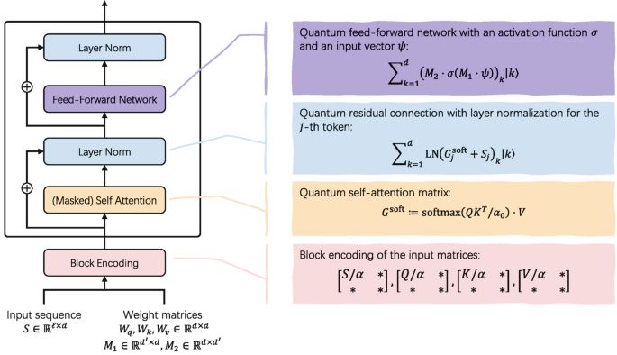
Figure : Quantum Transformer Architecture

 

Quantum Transformer : A 𝗾𝘂𝗮𝗻𝘁𝘂𝗺 𝘁𝗿𝗮𝗻𝘀𝗳𝗼𝗿𝗺𝗲𝗿 may sound complex, but conceptually it follows the same design as a classical transformer. The main difference is how computations are performed using 𝗾𝘂𝗮𝗻𝘁𝘂𝗺 𝗹𝗶𝗻𝗲𝗮𝗿 𝗮𝗹𝗴𝗲𝗯𝗿𝗮 instead of classical matrix operations. 

1. Input & Block Encoding: 

The model starts with: An 𝗶𝗻𝗽𝘂𝘁 𝘀𝗲𝗾𝘂𝗲𝗻𝗰𝗲 (tokens as vectors) 𝗽𝗿𝗲-𝘁𝗿𝗮𝗶𝗻𝗲𝗱 𝘄𝗲𝗶𝗴𝗵𝘁 𝗺𝗮𝘁𝗿𝗶𝗰𝗲𝘀 for attention and feed-forward layers Quantum computers can’t store matrices directly, so everything is converted into 𝗯𝗹𝗼𝗰𝗸-𝗲𝗻𝗰𝗼𝗱𝗲𝗱 𝗾𝘂𝗮𝗻𝘁𝘂𝗺 𝘀𝘁𝗮𝘁𝗲𝘀. This step enables matrix operations in the quantum domain. 

2. Masked Self-Attention: 

Just like in classical transformers, the model constructs: 𝗤𝘂𝗲𝗿𝘆 (Q) 𝗞𝗲𝘆 (K) 𝗩𝗮𝗹𝘂𝗲 (V) 𝗠𝗮𝘀𝗸𝗲𝗱 𝘀𝗲𝗹𝗳-𝗮𝘁𝘁𝗲𝗻𝘁𝗶𝗼𝗻 ensures each token only attends to 𝗽𝗮𝘀𝘁 𝘁𝗼𝗸𝗲𝗻𝘀, which is why this is 𝗱𝗲𝗰𝗼𝗱𝗲𝗿-𝗼𝗻𝗹𝘆. The attention scores are computed using a 𝗾𝘂𝗮𝗻𝘁𝘂𝗺 𝘀𝗼𝗳𝘁𝗺𝗮𝘅, and the result is stored as a 𝗾𝘂𝗮𝗻𝘁𝘂𝗺 𝘀𝘁𝗮𝘁𝗲. 

3. Residual Connection + Layer Normalization after Attention: 

The output is 𝗮𝗱𝗱𝗲𝗱 𝗯𝗮𝗰𝗸 to the original input (𝗿𝗲𝘀𝗶𝗱𝘂𝗮𝗹 𝗰𝗼𝗻𝗻𝗲𝗰𝘁𝗶𝗼𝗻) 𝗟𝗮𝘆𝗲𝗿 𝗡𝗼𝗿𝗺𝗮𝗹𝗶𝘇𝗮𝘁𝗶𝗼𝗻 (LN) is applied This improves 𝗺𝗼𝗱𝗲𝗹 𝘀𝘁𝗮𝗯𝗶𝗹𝗶𝘁𝘆 and 𝗶𝗻𝗳𝗼𝗿𝗺𝗮𝘁𝗶𝗼𝗻 𝗳𝗹𝗼𝘄, just like in classical transformers. 

4. Quantum Feed-Forward Network Next, each token passes through a 𝗳𝗲𝗲𝗱-𝗳𝗼𝗿𝘄𝗮𝗿𝗱 𝗻𝗲𝘁𝘄𝗼𝗿𝗸: 

Two 𝗹𝗶𝗻𝗲𝗮𝗿 𝘁𝗿𝗮𝗻𝘀𝗳𝗼𝗿𝗺𝗮𝘁𝗶𝗼𝗻𝘀 A 𝗻𝗼𝗻𝗹𝗶𝗻𝗲𝗮𝗿 𝗮𝗰𝘁𝗶𝘃𝗮𝘁𝗶𝗼𝗻 𝗳𝘂𝗻𝗰𝘁𝗶𝗼𝗻 In the quantum setting, these steps are implemented using 𝗾𝘂𝗮𝗻𝘁𝘂𝗺 𝗼𝗽𝗲𝗿𝗮𝘁𝗶𝗼𝗻𝘀, refining each token 𝗶𝗻𝗱𝗲𝗽𝗲𝗻𝗱𝗲𝗻𝘁𝗹𝘆.

5. Final Residual + Normalization Once again: 

FFN output is 𝗮𝗱𝗱𝗲𝗱 𝗯𝗮𝗰𝗸 𝗟𝗮𝘆𝗲𝗿 𝗡𝗼𝗿𝗺𝗮𝗹𝗶𝘇𝗮𝘁𝗶𝗼𝗻 is applied This completes 𝗼𝗻𝗲 𝗾𝘂𝗮𝗻𝘁𝘂𝗺 𝗱𝗲𝗰𝗼𝗱𝗲𝗿 𝗯𝗹𝗼𝗰𝗸.

Reference : Du, Y. et al. (2025). Quantum Transformer. In: A Gentle Introduction to Quantum Machine Learning . Springer, Singapore. DOI:https://doi.org/10.1007/978-981-95-1284-3_5